Think you’re diversified? Check your FX

Most investors carry FX exposure as a matter of course. This is a side effect of owning anything global. But few do anything meaningful with it. The risk is present whether you choose to engage with it or not. The conventional fix is neat: hedge it passively, reduce portfolio noise, and move on. But this misses the point. Passive hedging reduces volatility but leaves untouched the real potential of FX: returns streams that behave differently from equities and bonds, offering quiet diversification.

Currency markets are by nature fragmented, shaped by local macro cycles, shifting policy regimes, and geopolitical events. These forces rarely sync up across regions, and it’s this same misalignment that makes FX such a persistent diversifier. Trends in FX often evolve independently of traditional assets.

The practical trick is that you don’t need every currency to trend – just enough of them. Trend-following in FX is less about broad rallies, more about catching those scattered pockets of momentum when they emerge. The rest is left alone. Breadth is what gives this selective approach its resilience.

This third instalment of the Quanta Byte series on systematic FX looks at how that works in practice: how active trend-following turns passive FX exposure into uncorrelated alpha, why fragmentation is your friend, and what happens when you overlay an active FX basket onto something as simple as a global 60/40 Equity/Bonds Portfolio.¹

The Problem: Universal exposure, untapped potential

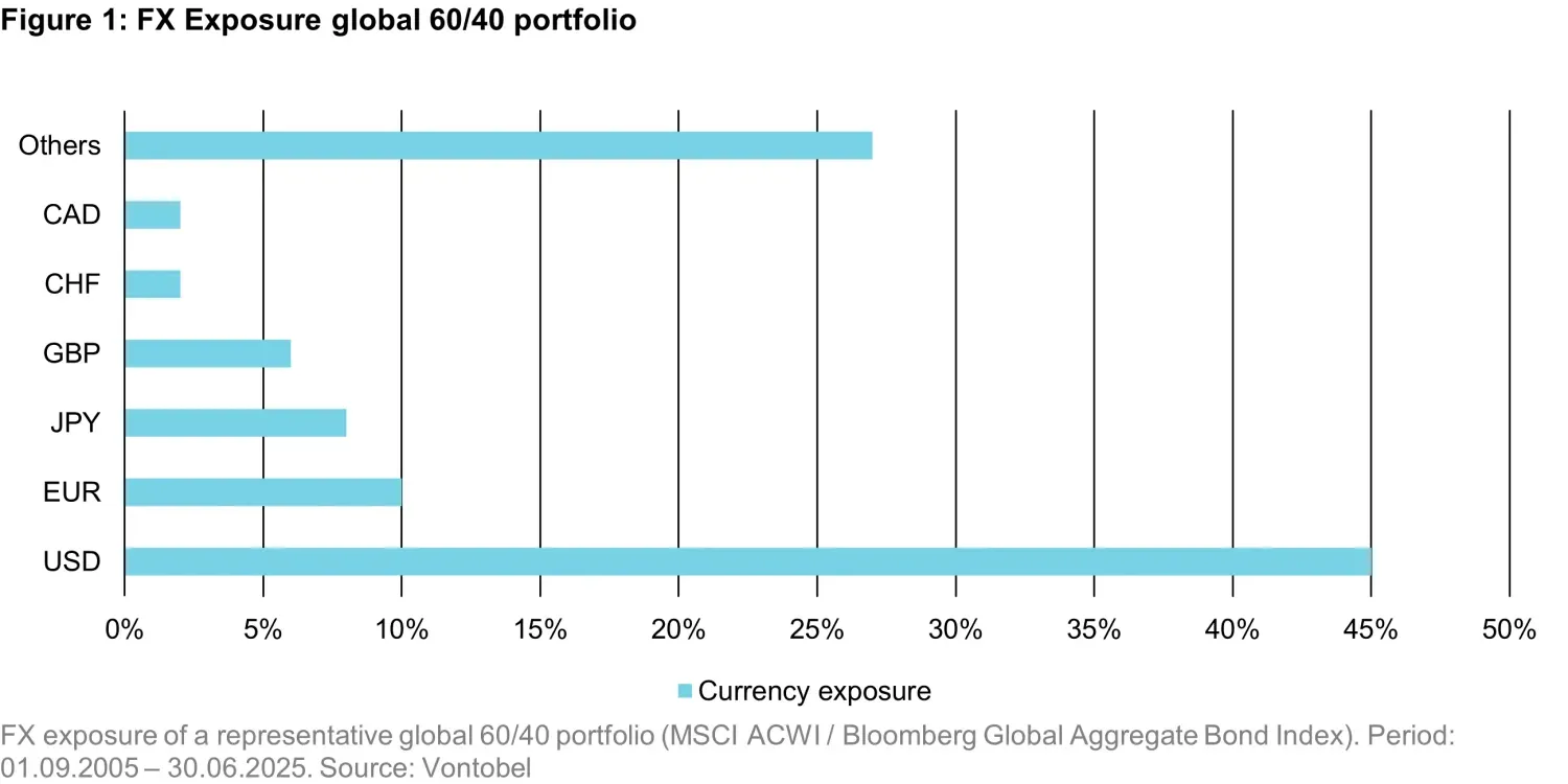
FX exposure is a near-constant feature of global portfolios. In a representative 60/40 allocation, whereby ‘representative’ is considered from the perspective of an investor measuring their wealth in USD, close to half of the underlying assets are denominated in non-USD currencies, as shown in Figure 1. This means that currency fluctuations can significantly affect returns, often for reasons unrelated to the core investment rationale.

The standard response is to hedge passively. This approach is straightforward and effective in reducing unwanted volatility. But it also eliminates any potential benefit from currency movements. The result is an exposure that becomes neutralized, yet still incurs costs — through hedge roll yields, transactions, and, most importantly, missed opportunity.

Hedging passively (or not, which is the other common decision) gives a false sense of security: it’s not because that you hedge systematically that you can rest assured that your portfolio behaves as you want. This is especially true nowadays when FX rates exhibit large swings.

Consider a CHF-denominated investor who invested in the S&P 500 during H1 2025. While the S&P 500 Total Return index had a good first half-year in USD, returning 6.20%, it returned -7.09% in CHF. That represents a 13.29 p.p. spread. It’s the difference between a good and a bad year, where the difference had nothing to do with equities.

Currencies behave differently from equities and bonds. They respond to local conditions — policy decisions, elections, geopolitical events — that are often idiosyncratic and asynchronous. This fragmentation creates return streams that are, at times, structurally uncorrelated. In practice, however, this potential is rarely used. And as we articulated in the extreme example before, not using it becomes a liability.

Volatility decomposition reveals the imbalance. In an unhedged portfolio, FX can account for a substantial portion of total risk. Yet the default treatment is to strip it out through hedging. But hedging is not diversification. True diversification draws on return streams that are not just uncorrelated in theory but genuinely independent in behavior across regimes. FX trends can offer precisely that. The structure of these trends, and how they contribute to diversification, is where we turn next.

The Engine: How FX trends unlock uncorrelated alpha

Not all trends are created equal, and indeed FX trends differ from trends in other markets. Currencies always trade in pairs, making all trends relative by construction: one currency strengthening means another weakens. There is no aggregate market direction like one might find in equities or bonds – just shifting relationships. This relative structure is key to FX trend-following. It doesn’t rely on broad market alignment but instead looks for local pockets of momentum. And because currencies respond to local fundamentals, such pockets emerge frequently, though not everywhere at once. This is where breadth matters. A diversified FX trend strategy doesn’t depend on widespread participation. It’s designed to capture isolated, independent moves as they arise. The more varied the basket, the more reliable the odds of finding such opportunities.

Consider a simple thought experiment: if each currency pair has a 50% chance of trending in a given month, then in a basket of 10, the chance of capturing at least three trends is close to 95%. This is based on a basic binomial model – but one that shows how fragmented trends can aggregate into something persistent. And our analysis supports this intuition. We apply a standard time-series momentum measure, inspired by the approach of Moskowitz et al. (2012)², that relies exclusively on an asset’s historical returns to generate a trend-following signal. For each currency i at time t, the signal S_(i,t)  is constructed as the average sign of cumulative returns over multiple lookback windows k , ranging from 1 to 12 months³. By construction, this approach captures sustained directional moves without relying on cross-sectional information or market-wide alignment.

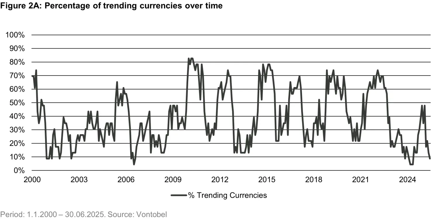
We evaluate the trendiness of currencies based on a sample of 23 developed and emerging market currencies measured against the euro⁴. As Figure 2A shows, the proportion of trending pairs fluctuates widely — from as low as 10% to as high as 80% between 2000 and 2025. This variability reflects the fragmented nature of FX momentum: some months deliver several strong trends, while others see only a handful.

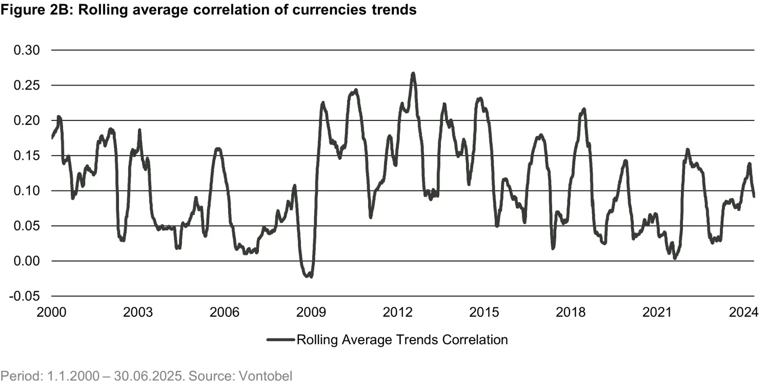
The empirical results highlight another key feature of FX trends: they are largely independent from each other. As Figure 2B shows, the average correlation of these trend signals across currency pairs remains low — typically between 0 and 0.2⁵. These low correlations are what make selective FX trend-following a robust diversifier, beating passive hedging every time. A passive hedge removes exposure entirely – along with any potential upside. A selective, active approach keeps the parts that matter: those that add uncorrelated return. Not every pair trends. Not every signal works. But enough do – and that’s the point. The value added? That’s up next.

The Payoff: What active FX trend harvesting does to a portfolio

The real test is portfolio-level impact. Does adding an active FX trend overlay improve outcomes in a meaningful way? The evidence suggests it does.

What makes active FX trend harvesting stand out is what it does to the risk-return balance when you bolt it onto something conventional, like a standard globally allocated 60/40 portfolio. Because the return streams from local currency trends are so often idiosyncratic, they show minimal correlation to equities and bonds, which is exactly what one is after when hunting for diversification that sticks.

A simple bit of maths backs this up. A single currency signal might deliver a Sharpe ratio of 0.3 – modest in isolation. But gather enough of these signals, keep their correlations low, and the basket’s overall Sharpe ratio improves materially. It’s the standard diversification toolkit: the more independent return streams at work, the lower total risk per unit of return. And a simple bit of practice shows it’s real. Simulate a basket of ten currency trend signals, each with a modest Sharpe and low cross-correlation. The combined Sharpe climbs well above what any pair can do alone – not because the signals are perfect, but because enough of them are imperfect and independent. That’s the point.

This effect shows up clearly when tested as an overlay. Take your standard global 60/40 portfolio for an EUR denominated investor and add an active FX trend basket on top. As shown in Table 1, by incorporating the FX trend-following overlay, the annualized return of the portfolio rises from 8.0% to 10.5%, while volatility increases only marginally—from 9.2% to 9.5%. The net effect is a significant boost in Sharpe ratio, from 0.82 to 1.05 and a cumulative total return that is 30% higher with respect to the classic 60/40 portfolio over the past 10-year period (Figure 3). Importantly, this enhancement is not the result of simple leverage or increased risk-taking; rather, it reflects the diversifying nature of FX trend strategies, which tend to perform particularly well during periods of macroeconomic stress and policy divergence.

The improvement is also robust across sub-periods and distinct macro regimes. During the pre-pandemic expansion (2015–2019), the Sharpe ratio rises from 1.14 to 1.28, while in the more volatile post-2020 period, it climbs from 0.65 to 0.92. In both environments, the FX trend overlay delivers consistent performance gains when added to the 60/40 portfolio. This persistence across both calm and turbulent regimes suggests that FX trends can capture risk premia distinct from those driving traditional asset classes.

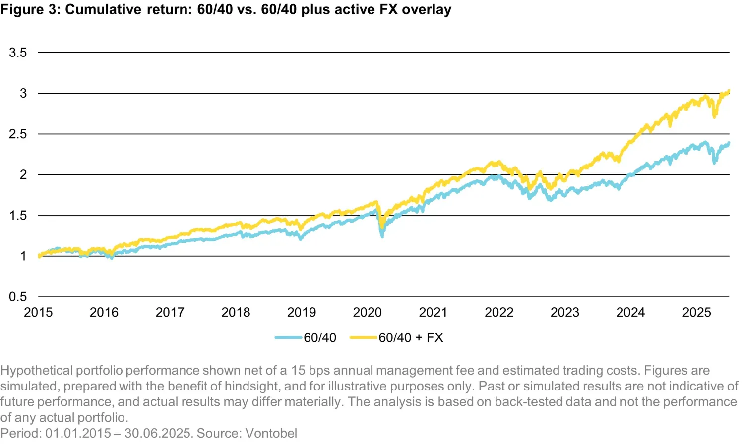
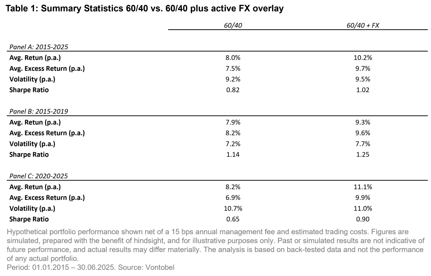
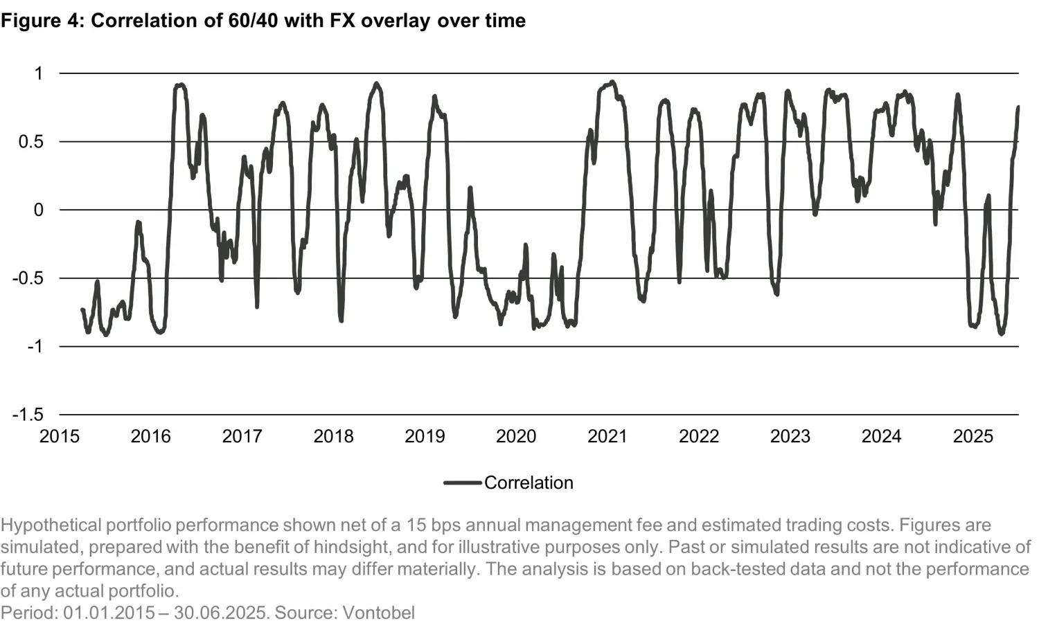
Figure 4 further illustrates the diversification benefits from another angle: the correlation between the 60/40 portfolio and our FX trend overlay is both time-varying and often negative. This makes FX trends a natural diversifier, offering returns that are largely independent of equity and bond cycles. Importantly, these strategies tend to deliver positive performance during periods when traditional portfolios struggle, providing both alpha potential and downside protection when it is most valuable.

Conclusion

FX exposure is inevitable for any globally invested portfolio. What remains is the choice of how to handle it. Passive hedging strips out volatility, but also discards return potential.

Active FX allocation, built around selective trend-following, takes the same exposure and reframes it: not as a nuisance, but as a source of uncorrelated alpha. The strength lies not in perfect prediction, but in disciplined breadth: collecting enough independent signals to let diversification do its work. FX doesn’t require alignment. Just enough divergence, across a wide enough set, to keep the return stream resilient.

Less is more. In FX, that means focused momentum, broad exposure, and patience. The result: diversification that does more than reduce risk — it adds value.