State-dependent risk

Compounding capital in financial markets is like ascending mountains. The rise can be steady and paced, but the falls are sudden and abrupt. It therefore makes sense to try and avoid those. Of all the metrics we look at as quants, one stands sovereign: volatility. Being able to forecast volatility is golden to protect the ascent.

In this article, we explore the challenges of accurately predicting volatility in financial markets and discuss the main limitations of traditional volatility models. We then introduce our State-dependent risk (SDR) model, a proprietary conditional volatility mode I designed to adapt more quickly to market conditions and address these limitations. We finally compare it against popular volatility models and demonstrate its forecasting performance.

Conditioning volatilities

Volatility represents the degree to which a security’s price fluctuates over a given period. Despite this simple definition, volatility is not directly observable and must be inferred from price movements using a statistical measure. The simplest and most widely used model calculates volatility as the standard deviation of returns over a fixed period—such as a month or a year – where all observations within that period are weighted equally. While intuitive, this backward-looking approach has significant shortcomings. First, this model struggles with capturing shifts in market conditions since its equal weighting scheme makes it slow to adapt to new volatility regimes. Moreover, it overemphasizes past extreme events, keeping the volatility estimates inflated for a long time after the stress periods have passed. Finally, the choice of the estimation window’s length is selected arbitrarily, and different windows can lead to significantly different estimates.

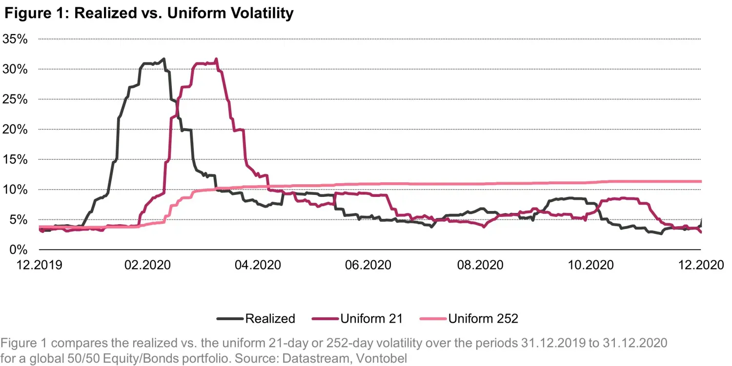
These issues become evident by comparing the 21-day and 252-day volatility estimates in Figure 1 during 2020 for a balanced 50/50 Equity/Bonds Portfolio. Both methods look backward, meaning they take time to catch up to the current environment, lagging behind realized volatility. This has important implications for portfolio managers. While the 21-day volatility reacts faster and is noisier than the 252-day counterpart, its lagging behavior can produce false signals, such as unnecessary trading in calmer periods or delayed responses when conditions worsen. Meanwhile, the longer 252-day window is more stable but clearly lags in recognizing major market turns and continues to reflect outdated volatility long after conditions have changed.

To address these shortcomings, conditional volatility models offer a more dynamic alternative to measuring risk. Conditional volatility refers to the expected volatility of an asset given past observations and information available at a specific point in time. This means that unlike the standard model described above, which treats past returns equally, conditional volatility models incorporate recent market conditions into their estimation process, allowing for a more responsive measure of risk. Additionally, conditional volatility models better capture the empirically observed property of volatility clustering, where high- and low-volatility phases persist over time. In the Systematic Multi-Asset team, we use a proprietary conditional volatility model called State-dependent risk (SDR) for risk-management. We believe the main strength of SDR lies in its ability to leverage not only the most recent data but also intelligently exploit insights from past market environments that are similar to the present, as we will now explain. The intuition here is that history repeats itself. Therefore, why not look at the most similar period in the past to inform what will happen tomorrow? Classical conditional models only look at the most recent past. But what if that was not representative of today’s condition? Our models seek to act on that.

Our proprietary model

The SDR model's principle is to assess how the current portfolio would react to the volatility patterns observed in historical data. The SDR’s volatility prediction follows a two-step process.

• First, we evaluate how closely the past resembles the present market conditions. How do we do this? We first analyze a wide range of factors that reflect the overall economic and market environment, such as interest rates, VIX and credit spreads. Then, using similarity measures, we compare today’s conditions with past periods to determine how much they resemble each other. The more a past market environment is similar to today’s, the more weight we assign to its data when estimating future volatility, unlike a standard volatility estimator that weights all past observations equally.
• In the second step, we look through historical volatility patterns: since we know the past, we have the advantage of being able to calculate the realized volatility for a given day that occurred over the next 21 days. By combining the dynamic weights of the first steps with these realized volatilities we are finally able to construct an expected similarity-weighted volatility for our current portfolio, which we label as SDR.

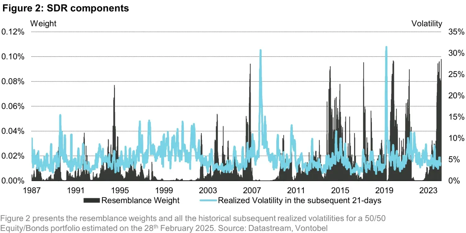
Figure 2 illustrates an example for the 28th of February 2025 using a 50/50 Equity/Bonds portfolio. On that date, the similarity measures estimated from the economic factors have determined a weighting scheme (represented by the vertical black bars) that was primarily loading on the recent years, mid 2010s and mid 2000s. Then, we calculate the realized volatility that occurred over the following 21-days for each of these days in the past, represented graphically by the light blue line. Finally, we estimate the SDR conditional volatility for the 28th of February 2025 as the weighted average of the blue using the black bars as weights, which yields a value of 5.64%.

SDR offers several advantages over conventional methods. First, it employs an "intelligent" measure that learns from past experiences, identifying patterns in historical data that are relevant to the current risk environment. This stands in contrast to fixed-window methods that treat all past observations with pre-specified weighting schemes. Second, as time progresses, SDR accumulates knowledge from an increasing number of similar periods, continuously enhancing its predictive accuracy and adaptability. Finally, SDR’s inherently dynamic incorporation of new information addresses the limitations of backward-looking traditional methods, effectively mitigating biases toward negative tail events discussed earlier. This is an important point. The recent past may be a good indicator of what will happen tomorrow, but it’s certainly not the best. Forecasting tomorrow’s weather by saying that it will equal today is better than a coin flip, but professional weather forecasting does markedly better. A similar dynamic is at play here.

In the animation below, we compare the forecasts of our conditional volatility model, SDR, against a traditional volatility forecast based on uniform data from the previous year. This comparison spans the period from 1999 to 2024 for a balanced 50/50 Equity/Bonds Portfolio. The results highlight SDR's inherently dynamic nature, in contrast to the slow-moving behavior of uniform volatility. During the two major crises, i.e. the Great Financial Crisis and the COVID-19 pandemic, SDR demonstrates a quicker downward adjustment. In contrast, the Uniform fixed-window model maintains elevated risk levels for an extended period, leading portfolio managers to overestimate risk long after the crises had subsided.

How accurate is SDR?

How can the visual patterns observed be translated into measurable forecasting accuracy? To assess this, one must evaluate how well the forecasted monthly volatility aligns with the actual realized volatility. This involves calculating the differences between predicted values and observed outcomes and using some statistical measures to quantify the accuracy of the model's fit. Table 1 presents key statistical metrics comparing the realized volatility of a balanced 50/50 portfolio with several commonly used volatility estimators. We compare SDR against five common volatility estimators: (1) the simple 21-day volatility; (2) the simple 252-day volatility; (3) RiskMetrics¹ (252 days, decay factor 0.94); (4) RiskMetrics (252 days, decay factor 0.98); and (5) Generalized Autoregressive Conditional Heteroskedasticity GARCH(1,1) with a 1,000-day estimation window².

These volatility models primarily differ in the weighting schemes applied to historical observations. Uniform volatility models assign equal weight to all past observations, either over the previous 21 days (monthly) or 252 days (annual). In contrast, RiskMetrics models apply an exponentially decaying weight, with the Decay 98 model exhibiting a slower rate of decay compared to the Decay 94 model. The GARCH model, on the other hand, applies a recursive weighting scheme that adjusts based on past volatility. Unlike equal- or decaying-weighting schemes, GARCH updates its volatility estimate by considering a mix between recent shocks (short-term persistence) and long-term trends in volatility. Lastly, our SDR model employs a dynamic weighting scheme that adjusts estimates based on the similarity between the current environment and past observations as explained before.

For all these models, we calculate the out-of-sample expected volatility for each day over a 25-year period, spanning from December 31, 1999, to December 31, 2024 in Table 1. Using five different models, we compare their predicted volatilities to the realized 21-day volatility. Forecasting accuracy is evaluated using standard metrics such as Mean Squared Error (MSE), Root Mean Squared Error (RMSE), QLIKE, and Mean Absolute Error (MAE). Additionally, in the lower part of the table, realized volatilities are regressed on a constant and on the predicted volatilities. In this regression, a beta value of 1 indicates an unbiased estimate under ideal conditions.

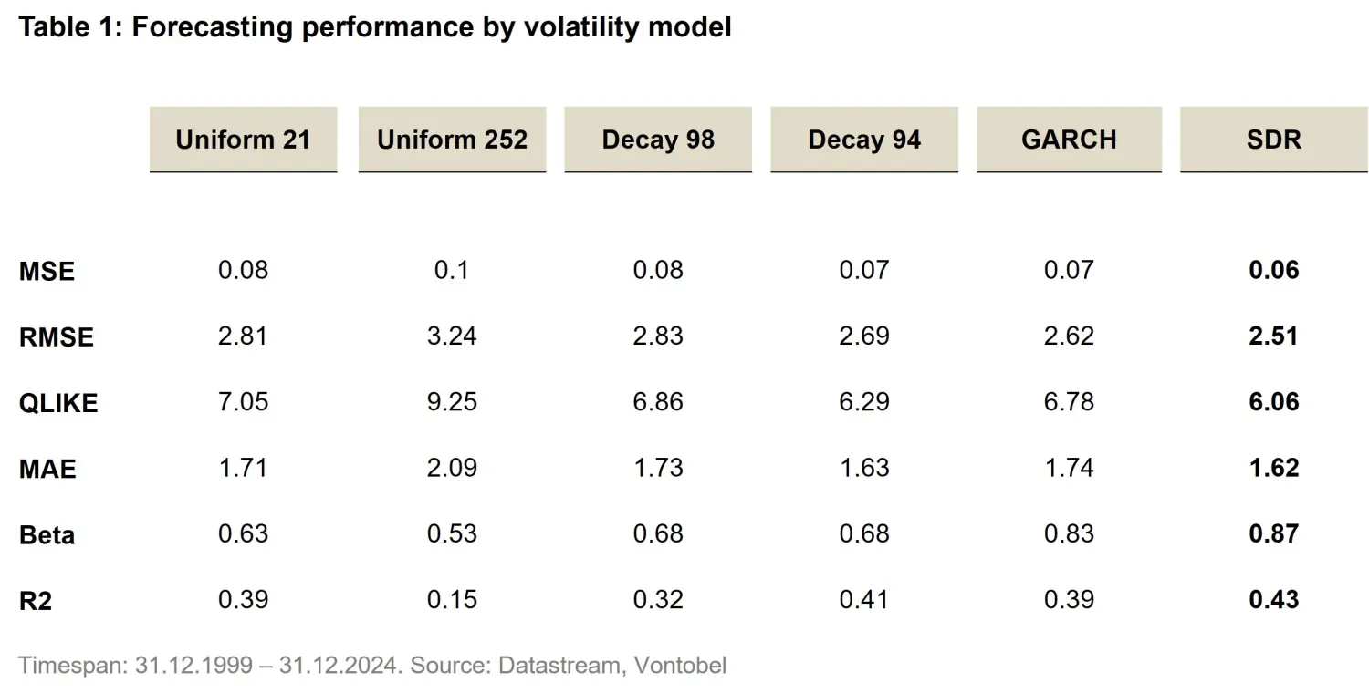
SDR consistently outperforms traditional models, including uniform, exponentially weighted, and GARCH(1,1) approaches, across all goodness-of-fit metrics. This indicates that SDR provides more accurate and reliable volatility forecasts compared to these established approaches. Furthermore, SDR achieves the highest beta value among all the models, reflecting its ability to deliver the most unbiased estimates of realized volatility under ideal conditions.

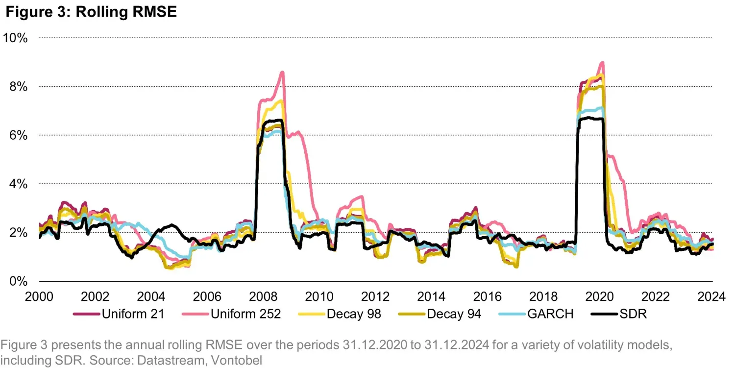
Figure 3 highlights the annual rolling RMSE statistics over the 25-year period. SDR maintains the lowest RMSE values for most of the timeline, underscoring its superior predictive accuracy. During the two major crises—the Great Financial Crisis and the COVID-19 pandemic—SDR exhibits significantly lower RMSE than other models and recovers more quickly following these market shocks. In contrast, traditional models, such as the 252-day simple volatility estimate, remain elevated for extended periods, causing portfolio managers to overestimate risk long after the crises have passed. SDR offers itself as a more effective risk management tool, by embedding all the main characteristics of a good volatility model. SDR remains, in fact, stable during normal market conditions, while reacting swiftly to stress periods. In addition, its progressive integration of data to its sample history allows it to avoid other shortcomings of traditional models such as the sudden loss of relevant historical information – which unlike fixed-window models is never removed from the sample - or the prolonged overestimation of risk after stress events.

Conclusions

We believe conditional volatilities provide a responsive measure of risk and SDR offers several advantages compared to conventional models. It simplifies calculations by avoiding optimization, instead leveraging an expanding historical horizon to learn from past conditions resembling the present, improving its predictive accuracy over time. SDR adjusts its weighting daily, staying responsive to current market environments while maintaining a dynamic perspective to anticipate shifts. By integrating historical patterns, and progressively expanding the sample size over time, it offers an intuitive and reliable measure of expected volatility. Empirical results confirm that SDR outperforms traditional models in forecasting accuracy, balancing agility in volatile markets with stability in calmer periods — enabling portfolio managers to scale financial peaks with confidence.

Important Information: The content is created by a company within the Vontobel Group (“Vontobel”) and is intended for informational and educational purposes only. Views expressed herein are those of the authors and may or may not be shared across Vontobel. Content should not be deemed or relied upon for investment, accounting, legal or tax advice.

Investment involves risk. Losses may occur. Vontobel makes no express or implied representations about the accuracy or completeness of this information, and the reader assumes any risks associated with relying on this information for any purpose. Vontobel neither endorses nor is endorsed by any mentioned sources.