Good old factors

1. Introduction

Welcome back to a new episode of the Expl(AI)ning series. In the last episode we saw that, despite AI’s wonders, we are far from seeing AI solve the very complex game of finance. And yet, AI has already made many contributions. Among those, it allowed us to improve on a well-known, broadly adopted, quantitative investment concept: factor investing in equities.

In this episode we will first review factor investing, discussing the impetus behind its genesis, and its evolution ever since. In doing so, we will re-affirm the explanatory power of factors, but challenge their forecasting capabilities, which ultimately matters when performance is the objective. Specifically, we will discuss three factor shortcomings: the need to time them, the limitations of their linearity, and their naïveté in forecasting.

2. A brief history of factor investing

Back in the early 1900s equity markets were highly ‘manual’, with only a handful of processes and structured data. Almost nothing was electronic, and price transparency was a challenge. Market moves seemed random, which unsettled many, and sparked curiosity in a few others. This latter group decided that it was worth their time to find ways to explain why and how the market moves.

Sharpe and Lintner^1,2 introduced the concept of beta, and were perhaps the first who found some structure in randomness. They observed that, while stocks seem to move up and down in sync with the broader market, some oscillate more wildly than others, and consistently so. Thus, they proposed to model an asset’s returns as:

\[ E(R_{i,t}) = R_{f,t} + \beta_i \left(E(R_{M,t}) - R_{f,t}\right) + \epsilon_i \tag{1} \] 

where \( R_{i,t} \) is the return of an asset \( i \) at time \( t \), \( R_{f,t} \) is the risk-free rate at time \( t \), \( R_{M,t} \) is the market return at time \( t \) and \( \beta_i \) is the sensitivity of the expected asset’s return to the expected excess market return.

Eq. (1) can be used to describe stock returns and simply proposes that the returns of a given stock \( i \) at time \( t \) can be expressed as the returns of the market \( M \) (at the same time \( t \)) multiplied by a coefficient beta, which is specific to the stock under consideration. In essence, Eq. (1) proposes a model where stock price movements are a linear function of market movements.

The researchers went on and tested Eq. (1) against reality, like any good scientist would do. Specifically, they tested whether, by feeding daily stock market returns in Eq. (1), a statistically significant beta could be found. And they did. Moreover, they found that a stock’s beta seemed to be persistent over time. That is, by re-running the same test a few years later, they found that stocks that had higher betas tended to still exhibit higher beta. Betas higher than 1 – as per Eq. (1) – denote stocks whose price oscillates more than the market. The opposite is true when beta is lower than 1.

Some sense in apparent randomness was found. Beta was effectively the first factor, later called the market factor. We say first factor because after testing Eq. (1) on real data, researchers also noted that the residual terms \( \epsilon_i \) were abnormally high. That is, while the model was able to capture some of the underlying structure, there was still randomness to be explained.

Not too long later, Fama and French³ proposed their three-factor model to further explain stock returns. In essence, they tested whether adding additional terms to the right of Eq. (1) (called regressors) could further reduce the residuals \( \epsilon_i \).

The main novelty was the addition of company specific characteristics to Eq. (1). The first was the company size, measured via its total market capitalization. The other was a form of value, a measure of how much a company is over or under valued versus its earnings and stock price. The intuition was simple, and the expectations clear. Consider size for example. Small companies tend to run more volatile businesses compared to larger companies. The smaller a company is, the apparent higher the chance that it will go bankrupt. This higher variability ought to be detectable via Eq. (1) when adding the size factor to the equation. Sure thing, results matched expectations. Similar arguments were made for value.

The combination of these three factors: size, value and market led to a higher level of return explainability, leaving less and less residual error. Still, this model was not perfect and could not explain all variance in the data.

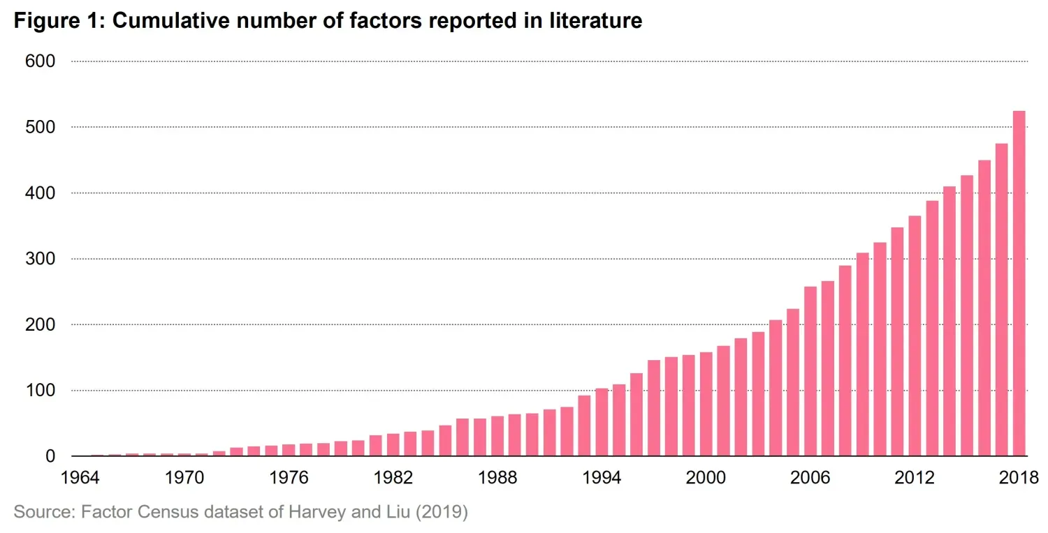
Researchers went on hypothesizing (and finding) one factor after the other. The academic literature on factors exploded and led to the definition of hundreds of ratios and indicators aimed at explaining returns. The result is shown in Figure 1, a phenomenon which many called a factor zoo⁴. A multitude of factors, all born to explain more and more returns in all possible market environments proliferated like mushrooms on a rainy day. Leaving cynicism aside, some withstood the test of time and became widely used. Beyond value and size, we are now accustomed to hearing discussions on the momentum, quality, and (low) volatility factors.

3. Investing with factors

Among the five factors listed above, quality shows peculiar resilience⁵. As a reminder: quality aims at identifying businesses that are stable and have sustainable profits. In this section, we will pick at quality to illustrate the main points of this episode.

Before we start, note that, unlike size, which has an almost unequivocal definition, the way we decide to measure quality is subject to interpretation. That said, the main pillars behind each quality definition are typically profitability (e.g., gross margin), efficiency (e.g., return on equity) and safety (e.g., leverage) metrics.

As most factors, quality is often used as part of an investment process to either select and invest in high quality companies (for instance by going long the top-quality quintile) or exclude low quality companies (for instance by going short the lowest quality quintile). But wait, what did just happen? In the section above we showed how factors can explain the variability of past returns. How did we make the mental jump to using factors as a way to select stocks that are poised to outperform in the future? We seem to misuse a variable that was originally conceived to explain the past in order to predict the future. Well, it turns out that the misuse is partially justified, and it’s got to do with some properties which factors exhibit over time.

Over the long run, factors have been shown to outperform the market, but what makes them truly valuable is a set of key properties that make them investable rather than just descriptive. Persistency ensures that their return premia don’t vanish overnight, while pervasiveness confirms that they hold across markets and asset classes. Factors also provide a risk premium justification, compensating investors for taking on systematic risks—though not all factors are created equal in this regard.

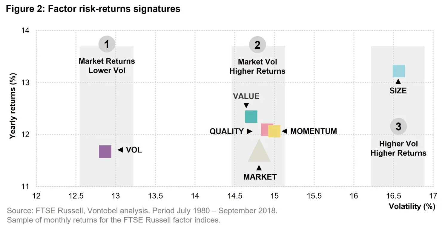
Moreover, factors exhibit low correlation, making them valuable in portfolio construction, and when they are robust and investable, they transition from academic concepts to practical tools for improving portfolio returns. As shown in Figure 2, each factor tends to have its specific mix of risk-return characteristics that constitute its unique signature and make it a good diversifier in a portfolio.

We identify three ways in which factors add value compared to the market. Firstly, a factor like (low) vol has delivered historical returns that are comparable to the market, but at much lower volatility. Secondly, factors like quality, value and momentum have delivered more than the market, with comparable volatility. Thirdly, size delivered more than the market, but with more volatility.

Armed with these insights, an investor that is more risk adverse will tend to drive towards (low) vol factors. Meanwhile, investors that are looking for high returns and can bear higher risk should look at size. This spectrum gives investors the chance to tune their portfolios and include factors based on their goals. It is also interesting to note that factors behave according to the mean variance theory by Markowitz. A factor that expresses a lower volatility tends to have lower returns and vice-versa.

Still, some factors raise an interesting question—are we truly uncovering deep market inefficiencies, or are we just formalizing the obvious? Take the size factor, for instance. Is it really a profound insight that small companies tend to outperform? After all, the small companies of today are the only ones that can become the big companies of tomorrow. Large caps don’t have the luxury of compounding from a tiny base. Yet, despite its tautological nature, size persists as a factor, much like value or quality. While its theoretical justification may be weaker than other factors, its historical performance and structural role in the market keep it relevant. This tension between genuine inefficiency and self-evident reality is part of what makes factor investing so fascinating—and occasionally, a little suspect.

We believe that the way factors are used to inform investment decisions is in fact not optimal, even if backed up by historical data and well affirmed in the industry. These indicators were initially created to help explain past returns and make sense of the chaotic behaviour we discussed at the beginning of the article. They have later been (ab)used in the industry as proxies to forecast returns and inform investment decisions⁶. We identify three core issues that naturally rise when in doing so. Firstly, there is a natural need for a timing mechanism that decides when to invest in each factor. While all factors seem to work over the very long run (as in: they do better than the market), sometimes the wait is unbearable. This prompts the need for investors to switch between factors frequently. Secondly, factors impose linear relationships by construction (see Eq. (1)), which is a major limitation in an inherently non-linear world like financial markets. And third, the way factors are used to forecast returns is based on a simplistic naïve assumption. Simply assuming that something that worked up until now is the best predictor for something which will happen tomorrow is a bit oversimplistic. We discuss these issues in detail in the next sections.

4. Timing factors

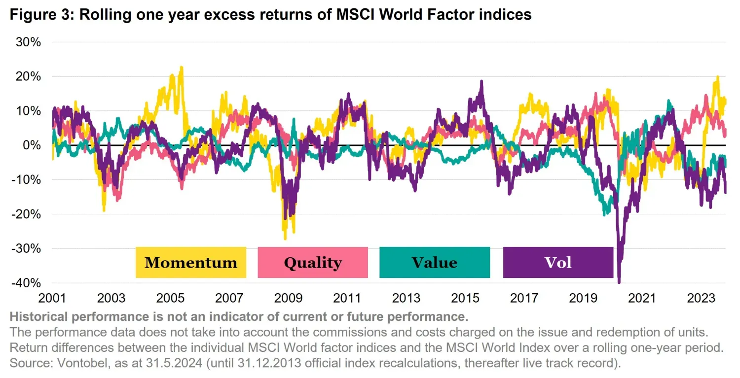
Factor performance varies across macro-economic regimes⁷. In Figure 3 we look at the evolution of rolling one year returns of 4 MSCI World Factor indices: momentum, quality, value and volatility. It is clear from the chart that there is no factor that always works. At first glance it looks like momentum and value are quite complementary but when looking closer we can see that there are periods in which this is not true. Picking one single factor and sticking to it is not ideal. It emerges that there is a need to decide which factor to use when.

Timing factors is hard and not always possible. In large global markets that are affected by a large multitude of parameters this might be close to impossible. Meanwhile in smaller markets such as Switzerland there are some characteristics that make it easier to try. The concentration of the market, the lower liquidity and the economic and geopolitical stability of Switzerland make it a good field to try and time factors. Still this is a solution that is not generalizable to any market or investment objective.

5. Linear expectations

Factor models, such as the Fama-French framework discussed above, assume a linear relationship between factors and expected stock returns. In the factor zoo spirit, let’s analyse the earnings per share growth (EPSG) factor. When using EPSG as a factor, this implies stock returns are modelled as:

\[ E(R_{i,t}) = R_{f,t} + \beta_i \left(E(R_{EPSG,t}) - R_{f,t}\right) + \epsilon_i \tag{2} \] 

where \( R_{i,t} \) is the return of an asset \( i \) at time \( t \), \( R_{f,t} \) is the risk free rate at time \( t \), \( R_{EPSG,t} \) is the return of a portfolio that invests by going long in high EPSG stocks and short those that have low EPSG at time \( t \). \( \beta_i \) is the sensitivity of the expected asset’s return to the expected return of the EPSG factor.

The formulation in Eq. (2) enforces a strict linear dependency between a stock’s returns and the EPSG factor returns. This is not the only linearity imposed by this model. The underlying hypothesis in the factor construction is that higher EPSG has the potential to yield higher returns and vice versa. In other words, we can say that a unit increase in EPS growth translates into a proportional change in expected returns.

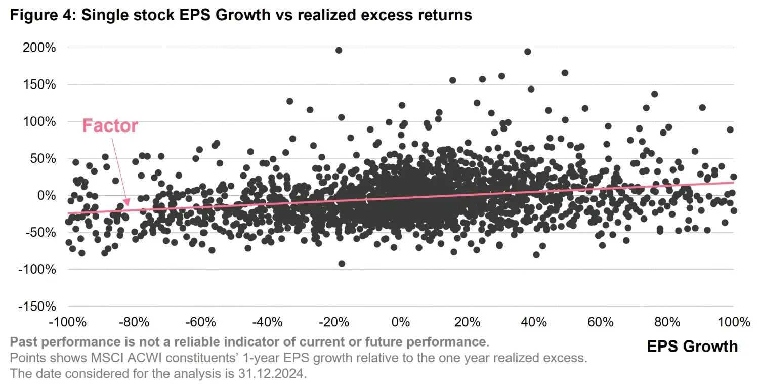
Figure 4 shows this relationship using real world data. Each point in the chart corresponds to a stock in the MSCI ACWI universe⁸. In this scatter plot we are able to show the relationship between EPSG and realized excess returns. We also qualitatively show how the factor would impose a linear relationship that is not obvious from the data (the straight line colored in coral).

The linearity assumption has significant limitations. Remaining on the EPS growth example, the relationship between EPS growth and returns is unlikely to be stable—growth stocks may be rewarded in certain market regimes (e.g., low-interest environments) but penalized in others. Second, non-linearities may emerge and remain uncaptured; for instance, extremely high EPS growth might indicate unsustainable expansion, triggering concerns about earnings quality or future mean reversion. Third, EPS growth does not act in isolation—interactions with valuation, profitability, or market sentiment introduce complexities that a simple linear model cannot capture.

By assuming linearity when building factor-based models the risk is to misrepresentreal-world dynamics which are better captured with moreflexible approaches—such as artificial intelligence or regime-switching models.

6. Naïve forecasting assumption

When using factors to invest as opposed to just explain past returns, we are implicitly making one assumption. Considering quality as example, this assumption reads: if investing in good quality worked yesterday, it will probably work tomorrow. This is not a bad assumption. After all, one of the best predictors of tomorrow’s weather is today’s weather. If it rained today, chances are it will rain tomorrow. In machine learning, we call this the naïve model. It’s the easiest thing we can say about the future without much effort. When we approach a problem with a machine learning toolkit, we always start by defining the naïve estimator. It serves as the bogey to beat. What one concludes is that factor investing lacks a forecasting effort by design. It simply tells you to invest tomorrow into what worked up until today.

Let us test if this is a sensible approach. Figure 5 depicts quality transitions in time, which allows us to answer the question: how likely is it that – if a company exhibited good quality up until now – that it will do so moving forward? To compile the analysis we used the S&P 500 universe over a period of 10 years, starting from 2015. From Figure 5 we observe that on average 72% of companies that are marked as “Very good” Quality (i.e., ranked in the first quintile) are remaining in the same quintile one year later. This is a very strong correlation. In fact, it’s the highest number in the table. Data are validating the hypothesis that past quality is a strong indicator of future quality. We conclude that after all, the naïve indicator is not that bad. Moreover, when measuring excess returns, we found that companies that are ranked “Very good” in the present (the whole first row of the matrix), on average, yield 50 bps excess returns during the following year. Incidentally, also notice that the second largest number in the table (i.e., the second strongest correlation) indicates that very low quality tends to persist over time. If 72% of the companies that were rated “Very good” remain “Very Good”, what happened to the other 28%? And by the same vein, who are the companies that ascended to “Very Good”, but weren’t “Very Good” up until now?

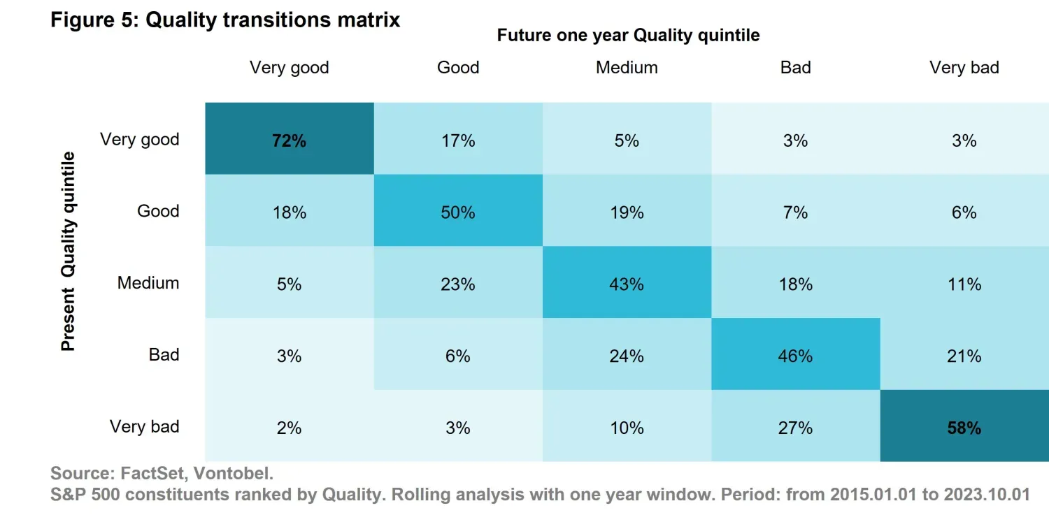
It turns out that companies that will have a “Very good” positioning in the future (the whole first column) yielded a weighted average excess return of 450 bps, which is 9x higher than the 50 bps associated with companies that are “Very Good” and will remain as such. These considerations lead us to conclude that the naïve estimator actually works but also that there is an opportunity that is left unaddressed by traditional factors. These insights are precisely what we strive for in our daily work with AI: moving beyond static, backward-looking metrics to dynamic, forward-looking predictions. By combining historical patterns with predictive modeling, we can uncover hidden opportunities and refine our understanding of what drives performance. In doing so, we transform raw data into actionable intelligence, enabling smarter decision-making and investment processes.

7. Conclusion

Factors are powerful methodologis that were developed to explain returns out of seemingly chaotic behavior. Further developments led to the misuse of these indicators, luring investors into using them to inform investment decisions. Factors present three core pitfalls that we described in detail: the need for a timing model, the imposed linear expectations between the factor and returns and the naïve forecasting assumption. Building on these points we believe that AI has the potential to recast factors under a new framework. With AI we could delegate to the model the choice of the most important factors, leverage the non-linear relationships of our problem and produce more accurate forecasts. This could give investors a look into the future while embracing the complexity inherited from the evolution of factors. In the next Quanta Byte of the Expl(AI)ning series we will propose an AI factor framework and discuss its advantages in detail.

1. Sharpe, W. F. (1964). Capital asset prices: A theory of market equilibrium under conditions of risk. Journal of Finance, 19(3), 425–442.
2. Lintner, J. (1965). The valuation of risk assets and the selection of risky investments in stock portfolios and capital budgets. Review of Economics and Statistics, 47(1), 13–37.
3. Fama, E. F., & French, K. R. (1993). Common risk factors in the returns on stocks and bonds. Journal of Financial Economics, 33(1), 3–56. DOI: 10.1016/0304-405X(93)90023-5
4. Cochrane, J. H. (2011). Presidential address: Discount rates. Journal of Finance, 66(4), 1047–1108. DOI: 10.1111/j.1540-6261.2011.01671.x
5. Asness, C. S., Frazzini, A., & Pedersen, L. H. (2019). Quality minus junk. Financial Analysts Journal, 75(1), 60–73. DOI: 10.1080/0015198X.2018.1547626
6. Ang, A. (2014). Asset management: A systematic approach to factor investing. Oxford University Press.
7. Fama, E.F., & French, K.R. (1989). "Business Conditions and Expected Returns." Journal of Financial Economics
8. MSCI ACWI Index Factsheet (accessed on 17.02.2025) https://www.msci.com/documents/10199/8d97d244-4685-4200-a24c-3e2942e3adeb