Backtesting Gone Wrong

“Past performance is not necessarily a reliable indicator of future returns.” – We read this warning so often that its meaning threatens to fade into the background noise. And yet the phrase strikes at a central conundrum of asset management: how can we distinguish real investment advantages from accidental success?

This question brings us to the practice of backtesting. By simulating historical performance, backtests allow investors to evaluate strategies before putting real money to work. But while indispensable, backtesting can also be dangerously misleading if not done with rigor.

That’s why we’re dedicating a two-part mini-series to the topic. In this first part, we explore why backtesting matters, illustrate it with a simple momentum strategy, and highlight the most common pitfalls that can distort results. In the second part, we’ll turn to what we believe to be best practices for designing more robust backtests and discuss how to transition from simulation to live trading.

Why Backtesting Matters

When deciding whether or not to invest in a particular investment strategy, investors like to look at the long-term performance of the investment vehicle. Although long-term live track records are clearly preferable as a basis for investment decisions, they are rare. Therefore, investors often rely on backtracked returns of the investment strategy in question. By backtesting an investment strategy, that is by replaying history with clearly defined investment rules and perfect discipline, decades of investment experience can be compressed into a few hours of computation time. This is indeed attractive. When done right, backtesting can:

• exclude weak ideas: The primary purpose of a backtest is negative in nature. In fact, by backtesting investment strategies, quantitative analysts and portfolio managers seek to discard investment strategies that are performing poorly, look fragile, or are capacity constrained (Arnott et al., 2019).
• frame realistic expectations: A Sharpe Ratio generated across multiple bear and bull markets is more meaningful than a point estimate from last month’s favorable or difficult market environment.
• identify operational weaknesses: Transaction costs, excessive portfolio turnover or unpleasant drawdowns are easier to discuss when the evidence is tangible.

However, none of these aspects is a guarantee of success. As Harvey and Liu (2020) argue, NO historical simulation should be taken as proof that an investment strategy will succeed in the current and future market environment. Therefore, backtest results of investment strategies can at best demonstrate that a particular investment idea is not obviously flawed.

Backtesting Flaws and Pitfalls

I Setting the stage: Backtesting a simple momentum strategy

To discuss and demonstrate the flaws and pitfalls of backtesting investment strategies, we consider a sample universe of five stocks (stocks A, B, C, D, E) over a period of four quarterly returns. At the end of the third quarter, stock E is delisted so that stock E can no longer form part of a common stock portfolio in quarter Q4. The stock returns considered in this Section are as follows:

Our goal is to develop a new momentum strategy for our model universe, consisting of stocks A, B, C, D and E. The investment strategy we want to analyze is as follows: At the beginning of each quarter, an equally weighted portfolio of the two best performing stocks in the previous quarter is formed and held until the end of the quarter. This simplistic momentum strategy for the cross-section of stocks in Table 1 yields the following quarterly returns (note that the “Strategy return” is the arithmetic average of the quarterly returns of the portfolio constituents):

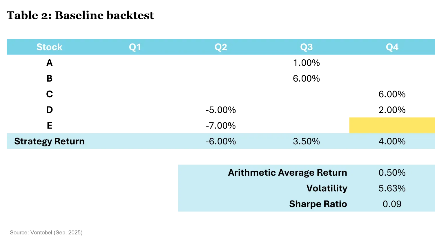
Table 2 shows that the proposed momentum strategy in our backtrack baseline scenario delivers an arithmetic average return of 0.50% per quarter, a quarterly volatility of 5.63% and (assuming a risk-free rate of zero) a Sharpe ratio of 0.50%/5.63% = 0.09.

Should we trust the results of our backtesting exercise from Table 2 and consider the backtrack results as a good predictor for the future performance of our momentum strategy? – The answer is YES and NO:

• YES, because our backtest has none of the flaws or biases we discuss in the upcoming Sections from II through V.
• NO, because the live track record of this investment strategy is likely to look worse due to transaction costs and market frictions.

To get a more realistic picture of the net performance of our momentum strategy, we next include transaction costs (outright trading costs plus bid-ask spreads) of, say, 0.5% per roundtrip trade in our backtesting exercise. In the case of our example strategy, all positions are only held for a single quarter, so that the portfolio turnover in each quarter is 100%. Therefore, the portfolio return net of transaction costs is reduced by 0.5% per quarter, and our momentum strategy yields an average return after costs of 0.00% per quarter and a Sharpe ratio after costs of 0.

Incorrectly considering transaction costs and market frictions is therefore a major reason why backtracked investment returns sometimes look better than the actual “live” performance of an investment strategy. However, as we show in Sections II to V, there are numerous other biases and pitfalls that can lead to a similar result.

II Look Ahead Bias

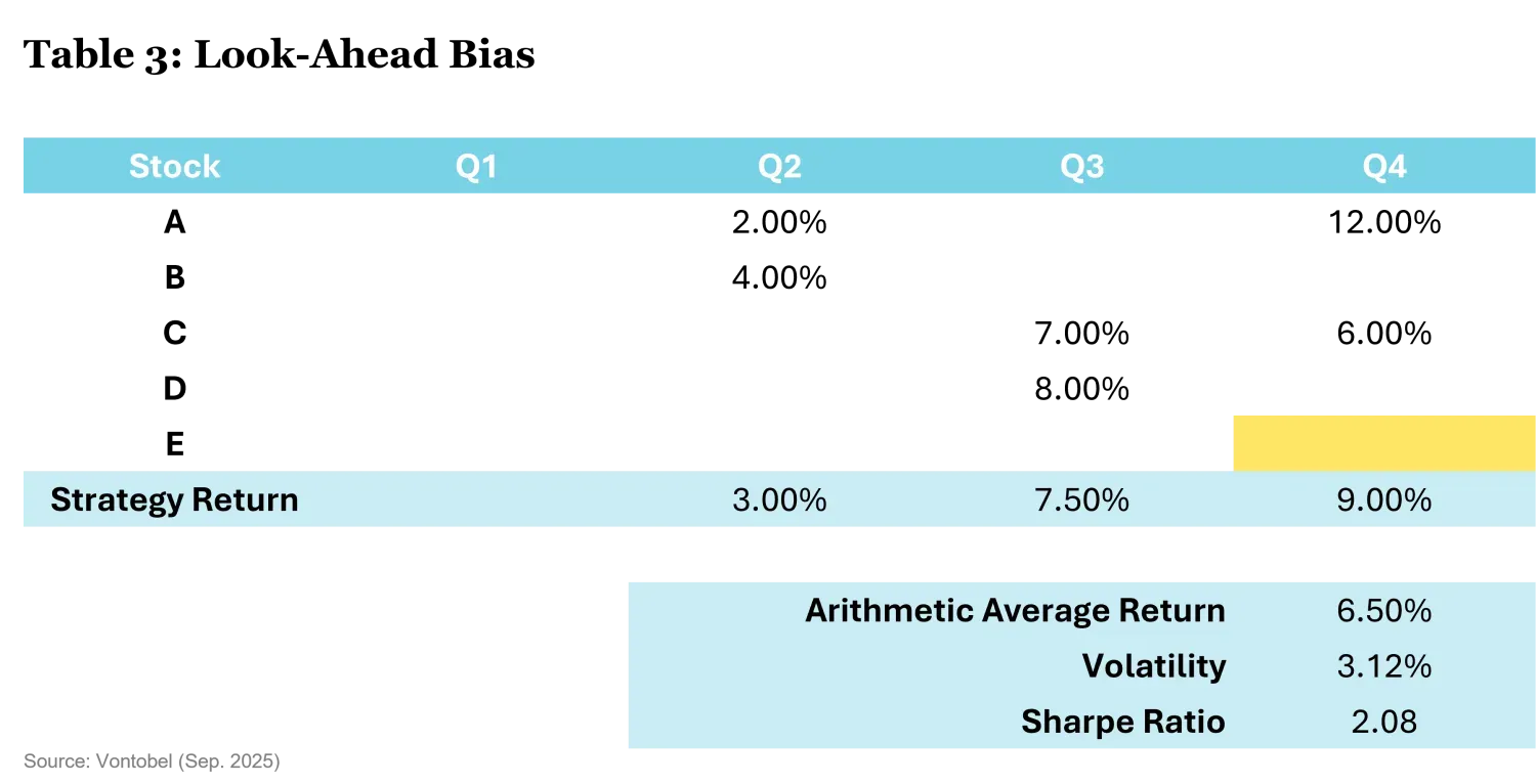
Using information that was unknown at the time of the actual investment decision is the main sin of historical simulation. In the case of our simplistic momentum strategy, we can introduce a look-ahead bias in our backtesting exercise by accidentally forming portfolios such that they contain the two best performing stocks in the current quarter (rather than the previous quarter). Failing to properly lag the information underlying the portfolio formation increases the arithmetic average return per quarter to 6.50% and the Sharpe ratio to 2.08, as shown in Table 3.

While the look-ahead bias in our example momentum investment strategy is easy to recognize, this is not always the case. Systematic investment strategies often rely on accounting data, which only becomes available with some delay and, in certain cases, is revised after the initial release. In principle, it is easy to eliminate the look-ahead bias. “Time-stamp” every input data with its first public release and then make sure that all input data is only used after this timestamp. Although this solution seems simple, it is often frustrating in practice as it slows down signal updates and shortens the time- series dimension of the sample data.

III Survivorship Bias

When creating a universe from the current cross-section of stocks, all companies that have gone bankrupt, merged or have been delisted are implicitly removed. Backtesting our example momentum strategy with the most recent cross-section of shares (i.e. the “survivors”) yields:

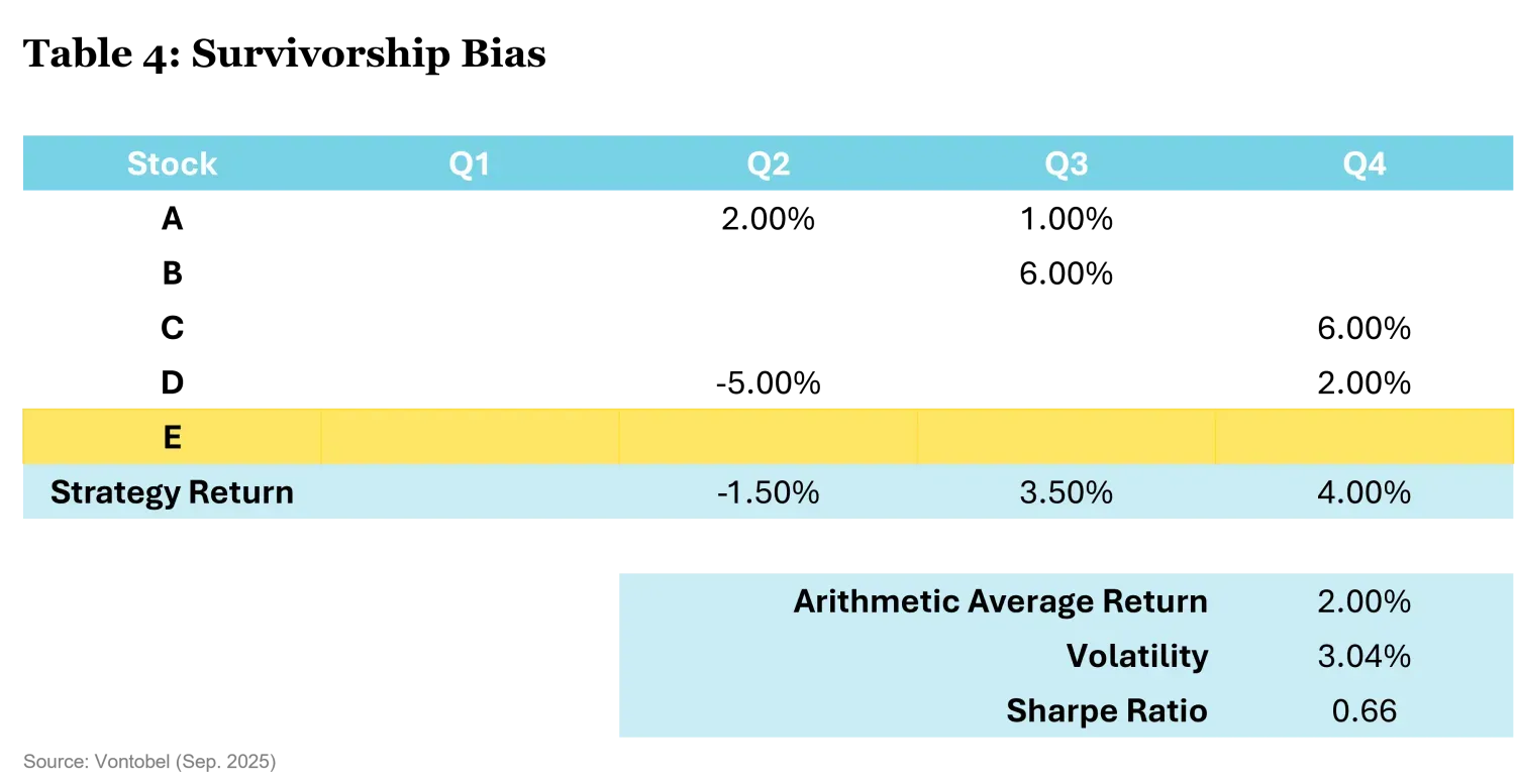
As can be seen from Table 4, both the arithmetic average return (2.00%) and the Sharpe ratio (0.66) are significantly higher compared to the backtesting of the example momentum strategy with the time-varying, actual stock universes. When backtesting investment strategies, it is therefore important to rely on a database that is survivorship-bias free. For US equity investors, the CRSP and Compustat databases are good examples of such databases, as they also contain securities that are no longer listed.

IV Data Snooping and Exhaustive Testing

In the 2010s, academic finance research documented more than 300 risk factors that predict the cross-section of average stock returns. Harvey, Liu and Zhu (2016) argue that once we account for the search intensity of identifying stock return predictors, the t statistic hurdle for declaring a new factor as a significant predictor for the cross-section of average stock returns should be above 3.0. 

Extensive testing can indeed be a major reason why the live performance of an investment strategy deviates from historical backtrack results. Testing multiple parameterizations of an investment strategy in a backtesting exercise is akin to adding more and more explanatory variables in a linear regression: The (in-sample) R-squared of the regression may improve, but the out-of-sample predictive power may actually worsen. Optimizing the parameterization of an investment strategy in a backtesting exercise is very tempting as it helps to “discover” an investment strategy that has worked well, at least in the past. Unfortunately, however, such “in-sample overfitting” (or data mining) of an investment strategy increases the likelihood that the actual live performance will be worse than the backtest results.

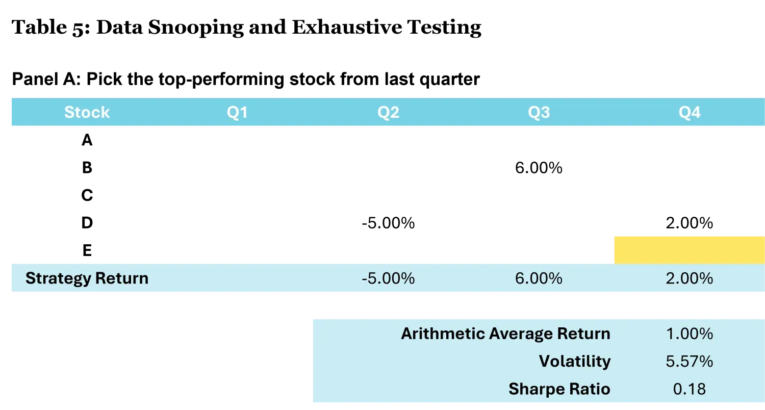
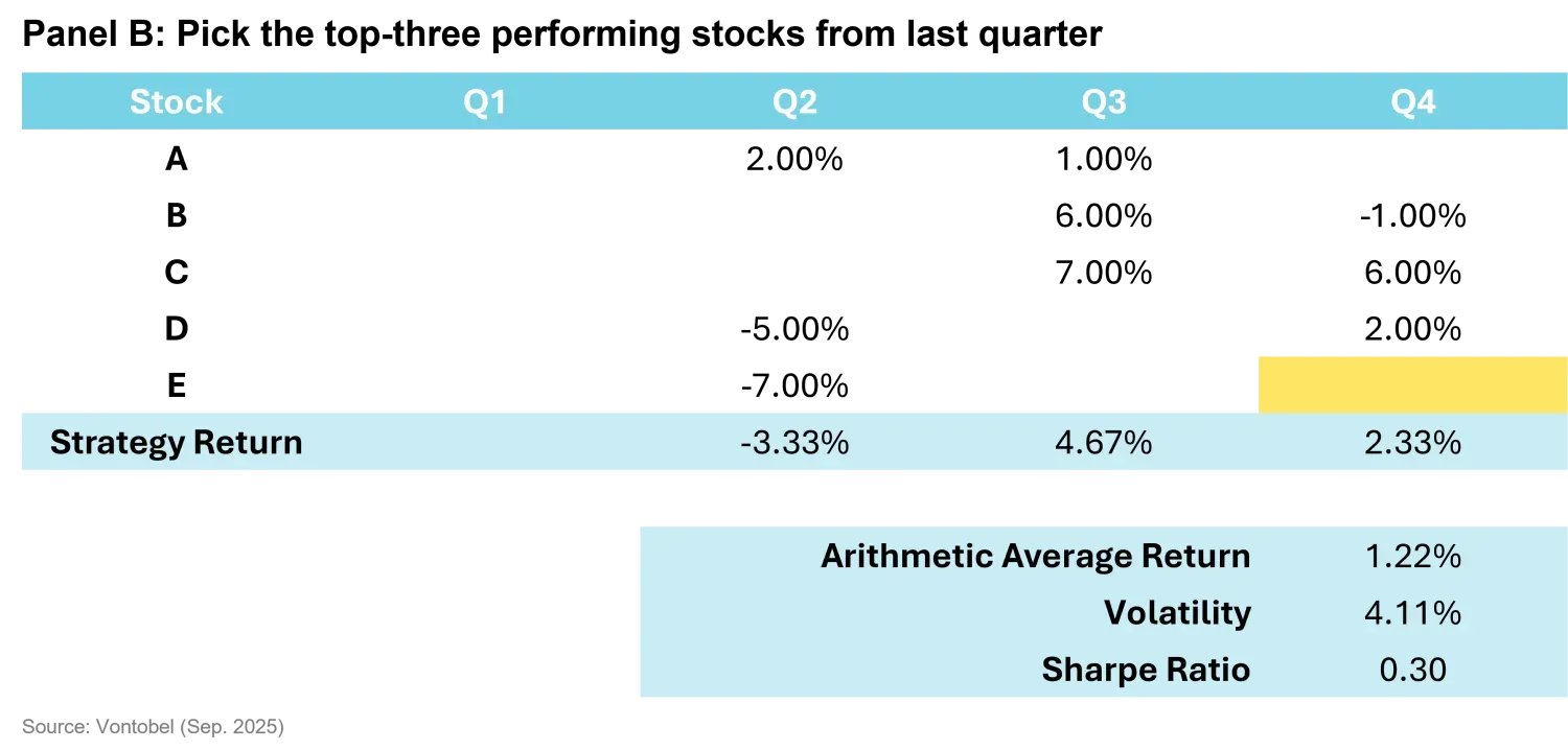
In the case of our simplistic momentum strategy, it seems tempting to experiment with the number of stocks in the momentum portfolio. In our base scenario, we have selected the two best performing stocks from the previous quarter. However, we could play around with this key parameter of our momentum strategy and instead invest in the single best performing stock of the last quarter (Table 5, Panel A) or in the three best performing stocks of the last quarter (Table 5, Panel B). Both these parameterizations improve the average return and the Sharpe ratio in the backtesting exercise, so we might be tempted to prefer one of these alternative parameterizations in the live version of our momentum strategy.

V Regime Dependence and Sample Period

An investment strategy can perform better in some market environments and worse in others. If the sample period of the backtesting exercise only covers a rather favorable market environment for the historically simulated investment strategy, the actual live track record may well look worse than that in the paper trading exercise – especially if the market environment changes.

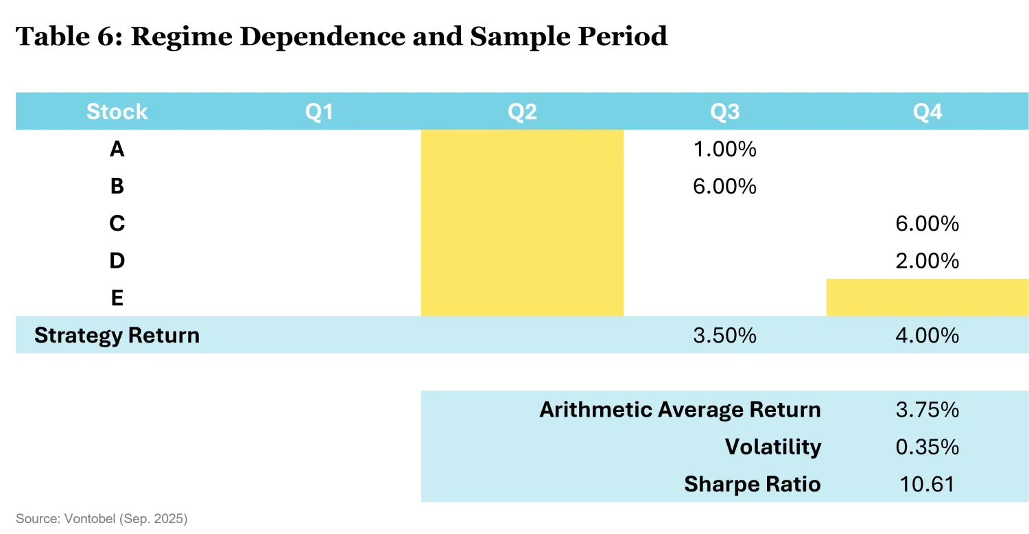
In our example, it is easy to see that the backtesting period plays an important role for the performance of the momentum strategy. If for some reason we limit the backtesting period to Q3 and Q4 (i.e. we start the backtest only after Q2), the arithmetic average return of the baseline strategy per quarter increases to 3.75% and the Sharpe ratio jumps to 10.61 (see Table 6 for details).

When developing an investment strategy, it can be tempting to limit the overall sample period to a more recent sub-period. In many cases, this may even make economic sense, as there may be good reasons why the market environment in the earlier part of the backtesting period was different from the current market environment. However, such arguments should always be carefully assessed to ensure that the sample period of the backtest is not inadvertently optimized. Playing around with the sample period is closely related to multiple testing: There is a risk that the backtracked performance of an investment strategy appears better than it actually is and that the actual live performance of the investment strategy therefore turns out to be worse than in the backtesting period.

Conclusion

Five imaginary stocks were enough to catapult the Sharpe ratio from 0.1 to 10.6 – simply by:

• Shifting timestamps – even a small misalignment between signals and prices can create the illusion of foresight.
• Ignoring delisted stocks – survivorship bias removes the losers and makes the past look far rosier than reality.
• Fine-tuning strategy parameters – over-optimization on in-sample data rarely translates into real-world performance.
• Restricting the backtesting window – carefully choosing start and end dates can turn weak strategies into apparent winners.

Just imagine the impact of the same shortcuts when the investment universe expands to thousands of securities and half a century of daily, monthly or quarterly data: Casual, unthoughtful backtesting can easily turn a seeming crystal ball into a hall of mirrors.

Backtesting is powerful, but also perilous if done carelessly. In this first part, we’ve seen how fragile results can be in the presence of biases and shortcuts. In Part II of this mini-series, we’ll move from pitfalls to practice: outlining best-practice principles that make backtests more reliable, and exploring how to bridge the gap between historical simulation and live portfolio implementation.

References

Arnott, R., Harvey, C. R., & Markowitz, H. (2019). A backtesting protocol in the era of machine learning. Journal of Financial Data Science, 1(1), 64 74.
Harvey, C. R., Liu, Y., & Zhu, H. (2016). … and the cross section of expected returns. Review of Financial Studies, 29(1), 5 68.
Harvey, C. R., & Liu, Y. (2020). False (and Missed) Discoveries in Financial Economics. Journal of Finance, 75(5), 2503-2553.
Important Information: The content is created by a company within the Vontobel Group (“Vontobel”) for institutional clients and is intended for informational and educational purposes only. Views expressed herein are those of the authors and may or may not be shared across Vontobel. Content should not be deemed or relied upon for investment, accounting, legal or tax advice. Vontobel makes no express or implied representations about the accuracy or completeness of this information, and the reader assumes any risks associated with relying on this information for any purpose. Vontobel neither endorses nor is endorsed by any mentioned sources.
About the authors
Daniel Höchle
Topics:
Read next:
2026 Large Language Models OutlookRelated insights
2026 Large Language Models Outlook
2026: Multi Asset Reloaded - Investors (Still) Need Diversification
Quant 2.0 - The AI Revolution
Global rates: a mirage of diversification
The signals beneath the surface