Machine Learning in FX: Learning the Unlearnable

Forecasting currencies remains one of the hardest challenges in systematic investing. FX markets are liquid, global, and influenced by fast-moving expectations. Yet they defy consistent patterns. Unlike equities, currencies rarely trend smoothly. Unlike bonds, they don’t follow fundamentals in a stable way. Instead, they react to relative surprises—policy shifts, data surprises, changes in positioning—and often do so with delay or asymmetry. Much of the time, the signal is weak and spread out across time.

Two characteristics make FX especially difficult to model: its sensitivity to sequence (i.e., their recent price behavior) and its structural instability. Both challenge conventional approaches that assume stable, contemporaneous relationships.

This final instalment of our Quanta Byte series on systematic FX explores how a specific class of machine learning algorithms – those that incorporate temporal memory – can offer a more fitting approach to the FX problem. For decades, currency markets have appeared resistant to prediction, not because they are fundamentally unknowable, but because available models assumed the wrong structure – static relationships, immediate effects, clean signals. FX has none of these. It is sequential, noisy, and shaped by lagged and relative surprises. We begin by exploring why sequence learning aligns more naturally with the temporal complexity of FX, and then turn to how instability – both in markets and in models – can be harnessed rather than avoided. In this light, learning the unlearnable is not a paradox, but a shift in perspective.

The failure of static models in FX

In 1983, Meese and Rogoff delivered a result that still defines much of the intellectual landscape in currency forecasting: even the most carefully specified structural macroeconomic models could not outperform a naïve random walk. This was not a matter of marginal underperformance. Even when the models were given future values of macro variables – an advantage bordering on clairvoyance which we call ‘cheating’ – they still lagged the assumption that tomorrow’s exchange rate will be today’s. The lesson was unsettling: the challenge in FX forecasting is not simply about refining the model or adding more data. It is tied to the very nature of the market.

The random walk remains the baseline to beat, and too often, it is not beaten at all.

This is not a failure of the more involved techniques themselves. It is a structural problem. FX returns are path-dependent, highly mean-reverting, and shaped by relative surprises rather than absolute levels. The signal-to-noise ratio is exceptionally low. Unlike equities, which can trend on fundamentals such as earnings or cash flows, and tend to go up over time, currencies lack intrinsic anchors. Their value is always relative, and shifts in price are less about discovering fair value than about digesting and sequencing shocks across economies. A rate surprise from the ECB, for instance, may dominate market attention only until a slightly larger surprise from the Fed reframes the narrative.

Understanding these structural features of FX brings us to the limitations of static models, which are poorly suited to such an environment.

By static models, we mean approaches that treat each observation as independent of its sequence. That means, these models take a single time-slice of data as input, ignoring patterns happening along the time direction. A regression or a random forest that uses today’s macro inputs to predict tomorrow’s return assumes that the past matters only through what is already captured in the latest data snapshot. It cannot distinguish between an inflation surprise that follows a series of upside beats and one that comes after months of downside misses, even though the market’s reaction to the two may differ sharply.
This limitation is particularly acute in FX. Consider the Eurodollar reacting to an inflation surprise. A static model may predict a similar effect in both cases, whereas a sequence model learns that the same surprise can have opposite implications depending on the preceding trajectory of data, commentary, and expectations. Context, in other words, is not an optional detail in FX. It is the entire mechanism through which signals become actionable.

A further reason why static models struggle lies in the signal-to-noise ratio. FX returns are notoriously noisy: even meaningful macro surprises can be overwhelmed by flows, risk sentiment, or cross-asset dynamics. Compared to equities, where fundamental information (earnings, growth) tends to dominate over time, FX signals are weaker, more dispersed, and often delayed. Empirically, this can be seen in lower R² values when regressing returns on fundamental factors, as well as in weaker directional predictability beyond the very short term.

Why sequence models work better

Traditional macroeconomic models are elegant but static. They tend to assume either stable relationships or immediate effects. And static machine learning models can further compound this effect by treating each observation as independent, ignoring the temporal nature of market dynamics. 
If asset dynamics depend on how information unfolds, then models should be able to learn from sequences. Most models, however, are static, i.e., they treat each observation in isolation. They ignore the sequence of events, the lag between cause and effect, and the structure of how information accumulates. In FX, this is a problem. Markets may react to events with delay. Positioning may build up slowly, then unwind quickly. Signals interact with each other over time, requiring models that can retain context over time.

The obvious mitigation is to include lagged features in the inputs of a static model. While this approach does in fact give the model orientation along the time direction, it quickly leads to an exploding number of parameters in the model: because every lagged feature gets its own parameter set, the total number of parameters scales with (number of features) x (length of lookback). For sure, one can add sparsely lagged features, but this immediately comes at the expense of lesser granularity.

So how can we have both a meaningfully time-oriented model and a controllable number of parameters? The answer is simple: share weights along the time direction, and let the model aggregate the obtained information for the final output. Recurrent neural networks (RNNs) – and their more robust variants such as LSTMs – are designed to implement this idea, as depicted in Figure 1.

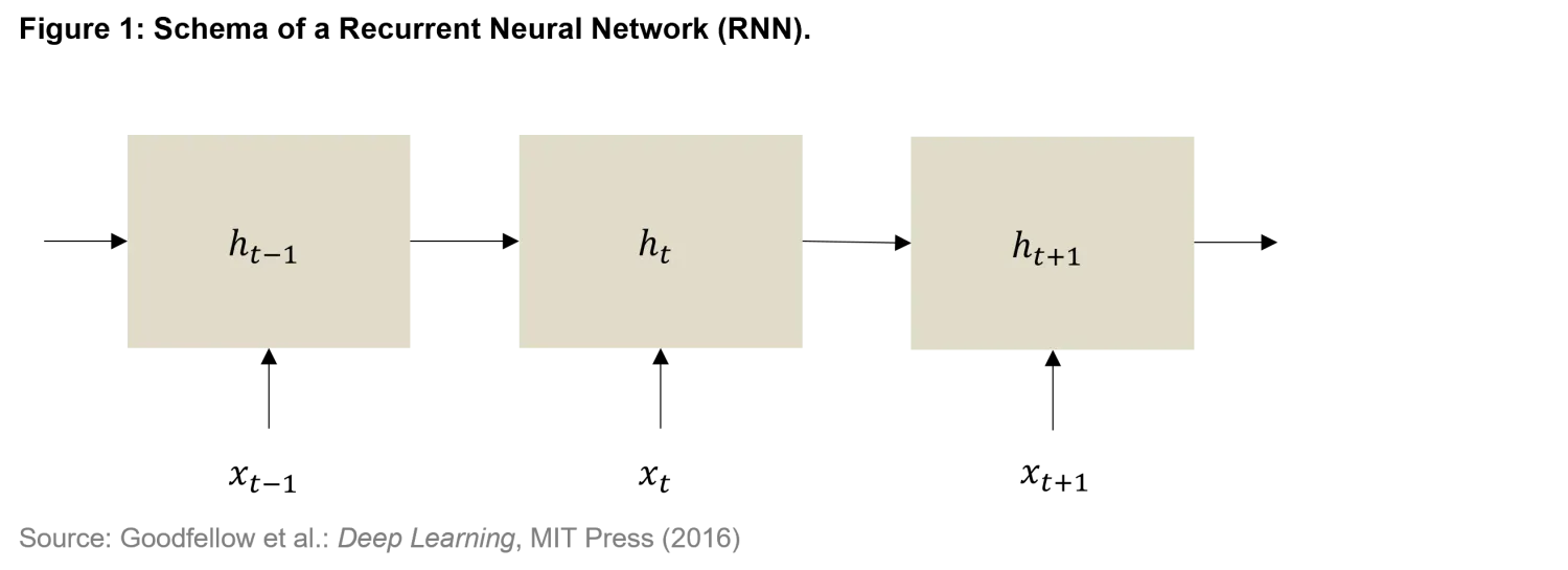
LSTMs address the limitations of RNNs by managing what information to retain or discard. They learn which parts of the past matter, and which can be ignored. This makes them especially useful for picking up patterns like lagged policy effects, delayed sentiment shifts, or decaying momentum. In our forecasting setup, each LSTM ingests a sequence of about 100 time series features and learns how historical configurations relate to future price direction. It does not impose assumptions about timing or relevance; it learns these from the data. This flexibility is further enhanced by so-called attention mechanisms. Rather than weighing the entire past uniformly, attention allows the model to focus on specific time points most relevant for the forecast.

Whether this added flexibility translates into better forecasts is ultimately an empirical question. Our live backtests suggest that it does. We evaluate model output by comparing monthly forecast accuracy to realized strategy returns. A positive relationship emerges: in periods when the model is more accurate, the strategy tends to perform better, and vice versa. This suggests that the model is not simply fitting noise. Its signals align, at least partially, with economically, meaningful variation.

This connection between forecast quality and return delivery offers a diagnostic check. LSTMs with attention don’t work in all conditions and certainly won’t guarantee success, but they offer something that traditional models don’t: the ability to learn how time matters.

Embracing instability

No single model consistently forecasts currency markets – least of all in foreign exchange, where the relationships between macroeconomic variables and asset prices shift frequently and often without warning. Machine learning does not resolve this problem in a conventional sense; instead, it reframes it. That reframing opens new possibilities, but it also introduces new complexities, particularly in how we think about uncertainty, learning, and robustness.

Even within a well-specified LSTM architecture, model outputs can vary materially from one run to another. Identical networks, trained on the same data with the same parameters, can yield distinct forecasts purely due to differences in random weight initialization. In many applications, such sensitivity might be viewed as a drawback. In FX, it reflects something deeper, namely, the instability of the problem being learned.

FX is structurally unstable. The dominant drivers of currency movements change over time, shaped by shifts in monetary policy, capital flows, geopolitical risk, or investor sentiment. At times, rate differentials might exert strong influence; at others, markets may be driven by positioning, liquidity demand, or risk-on/risk-off dynamics. This variability stands in contrast to asset classes like equities, where cash flows or valuations provide some anchoring mechanism. Currencies offer no such anchor. They are priced only relative to one another, and that relative pricing is continuously renegotiated by global macro conditions.
The connection between structural instability and model instability is not incidental. Neural networks trained on the same dataset but with different initializations tend to converge to different local minima. These represent functionally distinct but individually plausible models. In a high-dimensional parameter space, such divergence is expected rather than anomalous. Each model is shaped not only by the data it sees, but by the path it takes through the learning process. Small differences in starting conditions give rise to different interpretations – different "specializations" of the same underlying signal.

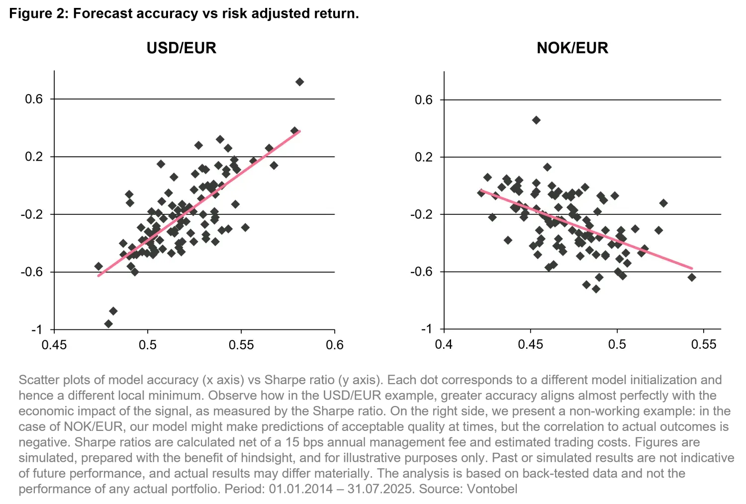
This phenomenon reflects a broader constraint: the limits to learning. In theory, with infinite data and a well-specified model, training would converge to a unique solution. In practice, data is finite, the signal-to-noise ratio is low, and the parameter space vast. The model improves during training but ultimately falls short of a global optimum. The result is a set of models that perform reasonably well out-of-sample but differ in the specific structures they internalize. These differences are not arbitrary, but rather reflect different, independently valid, views on how to react to a certain data input.

In a domain like FX, such diversity is valuable. A model that happens to learn a transient but dominant relationship may overfit. One that misses it altogether may underreact. Individually, both are brittle. But taken together, they form an ensemble that can better reflect the full range of plausible scenarios. Each model offers a perspective; but the ensemble builds a consensus. Where forecasts align, we have stronger reason to believe the signal is robust. Where they diverge, we gain insight into the limits of what can be known from the data.

Empirical evidence supports this intuition. Ensemble methods benefit and often encourage low average pairwise correlation between strategy outputs, (about 30% in our FX setup) building genuine variation in learned structure¹. Moreover, pairwise alpha tests between models reveal significant complementarity, with most pairs delivering positive alpha when used together. A tangency portfolio constructed across these model strategies, with no shorting and equalized volatility, tends to outperform any single constituent. These results underscore that ensemble complexity is not simply a hedge against model error; it can be structurally additive.

This is especially relevant in FX, where regime shifts are the norm and predictability is episodic. Under such conditions, robustness matters more than precision. An ensemble allows us to distinguish between idiosyncratic signals – those that arise in isolated model paths – and persistent ones that surface across diverse specifications. The goal is not to identify a dominant model, but to extract what remains stable across plausible variations . To illustrate this, we use average voting on an ensemble of 100 LSTMs forecasting AUD/EUR. As one can see in Figure 3, the performance of the 100 sub-models varies considerably, while the ensemble average displays a more robust behavior.

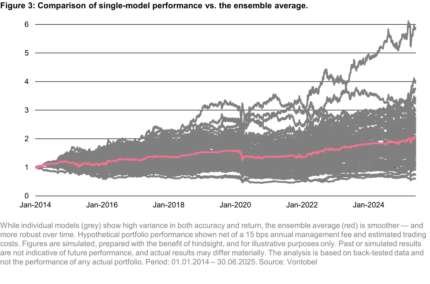
Viewed in this light, model instability is not a flaw to be corrected but a feature to be understood. It mirrors the structural instability of the underlying market and allows us to probe the space of possible explanations. Ensembles offer a principled way to navigate this uncertainty – not by resolving it, but by incorporating it into the learning process itself.

The resulting framework is not merely a technical improvement. It is a conceptual shift. Where traditional forecasting insists on singularity – a best model, a clean signal – the ensemble approach embraces multiplicity. It acknowledges the limits of inference in unstable domains and builds strength from pluralism. In FX, where instability is endemic, such pluralism is not just tolerable. It is essential.

Conclusion: to each its own

Machine learning does not simplify the task of forecasting currencies, nor does it eliminate the noise or uncover some hidden structure overlooked by traditional models. What it offers—when used judiciously—is a way to engage with markets on their own terms: as dynamic, fragile, and path-dependent systems where signals are fleeting and relationships unstable.

This is not a general claim. Different asset classes lend themselves to different methods. Where structure is persistent, and signals more clearly anchored, such as in equities or rates, simpler models may suffice. FX, by contrast, resists reduction. Its drivers are nonlinear, often delayed, and frequently regime dependent.

In that setting, sequential learning architectures like LSTMs with attention mechanisms that weigh context over time offer a better fit. They do not assume structure; they attempt to learn it. And when deployed as ensembles, they help surface patterns that are more likely to persist – not by filtering out noise, but by observing what survives across variation.

FX remains one of the more difficult domains for systematic prediction. That difficulty is not a deterrent, but a design constraint. It demands methods aligned with the nature of the problem, and a willingness to accept that robustness, not precision, may be the more realistic goal. Machine learning is no panacea. But in this context, it may just be the right tool.