Is this time different from 2007?

The present situation on the financial market shows ominous parallels with 2007 – at least according to our in-house risk-management model “State-Dependent Risk Measurement” (SDRM). The model suggests that we are in a market environment similar to the one before the financial crisis of 2007. According to one study, this crisis cost the global economy around USD 10 trillion and triggered one of the worst recessions since the global economic crisis of 1930. This is worrying, to put it mildly.

We did not have to wait long for this comparison to attract critics. The situation today is not comparable to the situation back then, the starting position is different, and the fundamental data do not match those of the phase before the financial crisis in any way, they said. The bottom line of the feedback is that this time everything is different. But is this true?

What are volatility clusters?

To shed some light on the matter, let’s take a look at the starting position and the data. The idea behind the SDRM is based on the knowledge that, since the beginning of the 1970s, various economic shocks and political upheavals have resulted in considerable price fluctuations followed by overreactions by market participants, which are reflected in volatility clusters¹. A characteristic of these volatility clusters is that they are repeatedly observed on the market independently of special events.² Intuitively, volatility clusters can be explained by the fact that price-relevant information resulting in a revaluation of securities does not tend to emerge at steady intervals over time, but rather clustered within short periods as a result of particular events.³ This effect results in volatile and calm market phases.⁴

How does the SDRM model work?

The identification of historic volatility clusters similar to the current market situation can help to better estimate the expected volatility and thus the current market risk in the short and medium term. To this end, the SDRM model – similarly to an image recognition algorithm – compares the current financial market environment with snapshots of the past. In doing so, it tries to identify the image in the historic financial market that most closely matches today’s situation. In the SDRM model, the market environment is represented by a total of seven state variables: dividend yield, credit spread, TED spread, term spread, short rate, VIX and MOVE index.

Macroeconomic drivers or vulnerabilities that result in market distortion are seldom directly comparable. There are significantly correlations in the transmission of shocks in the financial market via the said financial market variables. When identifying a historically similar market environment, we therefore expect much greater success with the “financial market approach” than with the “macroeconomic” approach, in which a comparable economic environment is sought.

The similarity of the current market environment to historic market phases is determined using the “nearest neighbor” approach, which searches for the smallest distance or rather the lowest difference of each state variable from its historic values. As soon as these “economic neighbors” are identified on the basis of the weighted distance between the state variables and today, the SDRM uses historic data to model the expected volatility for the next 21 days.

Are we experiencing déjà vu?

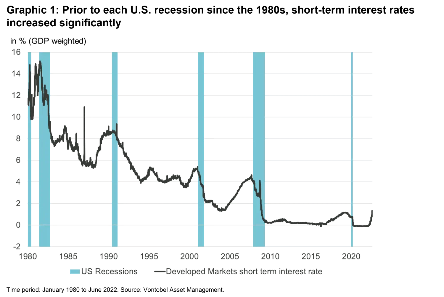
In recent weeks, the SDRM model has noticeably increased the weighting of the phase before the financial crisis of 2007. This means that the model is increasingly finding similarities with data points from this period. Currently, for example, the short-term interest rate or price of liquidity is increasing at a similar rate as in 2007. The change in this state variable has often been a precursor to a deep recession (chart 1) and low equity yields, such as in the run-up to the recessions of the 1980s, 1990s, and 2000s. This is also supported by the fact that both the US Fed and the Bank of England are currently pursuing the most aggressive cycle of interest rate hikes in several decades.

However, a look at the fundamental data shows that a repeat of the financial crisis of 2007 is rather unlikely. Over recent years, the International Monetary Fund (IMF) has repeatedly identified risks for companies in emerging markets, especially in the Chinese real estate industry⁵ and in the leveraged loans sector, but a strong de-leveraging process has begun since the financial crisis, especially in US households. This reduced the debt ratio as against the phase before the financial crisis. Moreover, the equity regulations of Basel I-III mean that banks now have to take fewer risks or that risk provisioning has improved. Accordingly, the current state of the finance industry does not unequivocally suggest that it could end in a financial crisis. However, in the current environment we are finding certain abnormalities that, taking historic data into account, signal increased stress in the financial market and urge caution.

Steady increase in credit spread since start of year

It is conspicuous in comparison with the market situation of 2007 that, in addition to the short-term interest rate, the credit spread, which measures market participants’ confidence in the solvency of companies and their refinancing options, has also increased. This is no surprise given the aggressive monetary policy, as it increased the recession risk in developed markets. During an economic downturn, credit risk premiums rise as a result of higher credit risk. Their increase is amplified by the flattening of the yield curve.

The current tightening of monetary policy, which had been extremely loose for ten years, coupled with a global economic downturn associated with declining corporate profits, is resulting in growing risks for certain sectors, such as the Chinese real estate industry. The increased costs of refinancing and the declining credit ratings of such companies are reflected in higher credit spreads. The same development was also observed ahead of past recessions (chart 2). The credit spread has increased to 1.8% since the outbreak of the Ukraine crisis and is now at a similar level as in 2007. However, it is still a long way away from the high of the financial crisis (4.9%).

For us, the signal of rising credit spreads is an important indicator of the future development of the real economy and potential risks. In addition, it should be noted that significant fluctuations in credit spreads disrupt the correlation between short-term interest rates and real economic activity.

Revision of long-term growth forecasts in current market environment

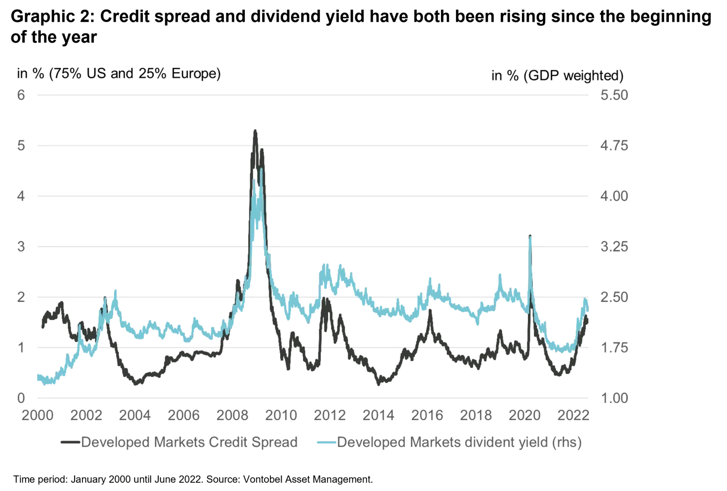
During the Great Recession of 2007-09, both credit spreads and equity markets were subjected to considerable financial tensions.⁶ This put significant strain on real economic activity and the business cycle. Widened credit spreads and collapsed equity prices also characterized the recessions of 1990/91 and 2001. As a rule, a slump in equity prices reflected in rising dividend yields is accompanied by a widening of credit spreads. This is also shown by the S&P 500, which has dropped -20% since the start of the year. Equity markets only saw a greater loss in the first half of the year during the Great Depression of 1932 (-40%) and in 1962 (-22%).

Equity market downturns are largely determined by the discount rate that rational investors apply to profits and the expected future profit growth.⁷ Since the COVID-19 downturn, however, equity returns have instead been influenced more by changes in the long-term expected dividend growth than by a change in the discount rate.⁸ In the current environment with sharply rising inflation, it is apparent that these high expected returns⁹ were not due to “better” technology, but the flood of cash unleashed by central banks.

In the environment of low interest rates and the glut of liquidity from the central banks, since 2020 investors have also been buying equities with low or negative dividend yields. They were led to this irrational behavior by the hope that the companies would “grow into” the expected cash flows on the basis of the anticipated dividend growth. Especially in the technology sector, these profit expectations are exceptionally high.

We saw the potential consequences of this overestimation of future growth prospects in investment decisions on the financial market in the first week of February. On February 2, 2022, a market value of USD 240 billion, roughly equal to the Swiss pharmaceutical giant Novartis, was wiped off the New York Stock Exchange within a day.¹⁰ This collapse was triggered by one company, and the reason seems rather trivial: For the first time in its 18-year history, Meta Platforms – formerly Facebook – reported a decline in the number of its active users by around one million. Given the fact that the social network has around 1.93 billion daily users worldwide, the question from a rational perspective is how a 0.05% decline in user numbers can justify a price slump of nearly 26%.

Other technology stocks such as Netflix, Amazon, Microsoft, and Apple have also lost large portions of their market value since the beginning of the year. What we are currently seeing in the market is a classic valuation correction at the end of a cycle that was driven by hope and the flood of money from central banks. This development can also be seen in the dividend yield, which has been steadily increasing in our model since the start of 2022.

Conclusion

The parallels with the phase before the 2007 financial crisis revealed by our SDRM should not be interpreted as a prediction of the next financial crisis. The model lacks indicators of the measurement of macroeconomic vulnerabilities, such as leverage, to estimate system risks and identify contagion risks. However, the presented comparison suggests that we are very likely to remain in a similar volatility environment to that of 2007 for the time being.

The strength of the SDRM is that it can use the identified volatility cluster of 2007 to help identify a risk profile for the next 21 days and thus derive the risk-appropriate asset allocation that can potentially perform best in this “economic neighbor period.” It thereby seeks the optimal balance between reactivity in tough market phases and a steady hand in normal market phases – typically a contradiction in risk management.

DISCLAIMER:

The views and opinions herein may change at any time and without notice. Such information is not intended to predict actual results and no assurances are given with respect thereto. Certain information herein is based upon forward-looking statements, information and opinions, including descriptions of anticipated market changes and expectations of future activity of countries, markets and/or investments. We believe such statements, information, and opinions are based upon reasonable estimates and assumptions. Actual events or results may differ materially and, as such, undue reliance should not be placed on such forward-looking information. Vontobel reserves the right to make changes and corrections to the information and opinions expressed herein at any time, without notice. This article is not an offer to sell or the solicitation to buy any security. It does not constitute a recommendation to buy or sell any security. Past performance is not necessarily indicative of future performance, future returns are not guaranteed. There is no assurance that the adviser will make any investments with the same or similar characteristics to the investment presented.
 

1. Such insights, which are empirically observed but not theoretically established, are also referred to as “stylized facts.”
2. Schmid, F. & Trede, M. (2006). Finanzmarktstatistik. Berlin Heidelberg: Springer.
3. Engle, R. (2004). Risk and volatility: Econometric models and financial practice. The American Economic Review, 94 (3), pp. 405-420.
4. This characteristic is also referred to as conditional heteroscedasticity.
5. International Monetary Fund (2021). Global Financial Stability Report, October 2021, retrieved from https://www.imf.org/en/Publications/GFSR/Issues/2021/10/12/global-financial-stability-report-october-2021
6. Brunnermeier, M. K. (2009). Deciphering the liquidity and credit crunch 2007-2008. Journal of Economic Perspectives, 23 (1), pp. 77-100; Adrian, T. & Shin, H. (2010). Financial intermediaries and monetary economics, in Friedman, B.M. & Woodford, M. (eds), Handbook of Monetary Economics (Vol. 3) (pp. 601-650). Amsterdam: North Holland.
7. Campbell, J. Y., Giglio, S. & Polk, C. (2013). Hard times. Review of Asset Pricing Studies, 3(1), pp. 95-132.
8. Böni, P. & Zimmermann, H. (2021). Are stock prices driven by expected growth rather than discount rates? Evidence based on the COVID 19 crisis. Risk Management, 23(1). pp. 1–29.
9. The expected return is calculated according to the Gordon growth model with the formula k=D0/P0+g. Translated, this means that the return with which an equity is sold equals the current dividend divided by the current price (dividend yield) plus the expected growth rate of the dividend (g).
10. In absolute charts, this is the biggest decline in a company’s market value of all time.